 .
.
![]()
|
|
|
|
|
|
|
|
|

The patterns of settlement in Early Christian County Down
Table 8
Chi-squared values for each altitude zone
|
Site type |
Altitude zone, in metres |
Chi –sq. |
|||||
|
. |
|
|
|
|
|
|
. |
|
Rath |
|
|
|
|
|
|
|
|
Probable rath |
|
|
|
|
|
|
|
|
Platform rath |
|
|
|
|
|
|
|
|
Raised rath |
|
|
|
|
|
|
|
|
Rath and souterrain |
|
|
|
|
|
|
|
|
Large rath |
|
|
|
|
|
|
|
|
Conjoined rath |
|
|
|
|
|
|
|
|
Rath pair |
|
|
|
|
|
|
|
|
Bivallate rath |
|
|
|
|
|
|
|
|
Multivallate rath |
|
|
|
|
|
|
|
|
Large enclosure |
|
|
|
|
|
|
|
|
Cashel |
|
|
|
|
|
|
|
|
Crannog |
|
|
|
|
|
|
|
|
Mound |
|
|
|
|
|
|
|
|
Souterrain |
|
|
|
|
|
|
|
|
Ecclesiastical sites |
. |
. |
. |
. |
. |
. |
. |
|
Pre-Viking |
|
|
|
|
|
|
|
|
Pre-Norman |
|
|
|
|
|
|
|
|
Probably pre-Norman |
|
|
|
|
|
|
|
Individual values become significant at 3.8.
Overall chi-squared vales become significant at 11.07
By applying the chi-squared test to the distribution of the ecclesiastical sites throughout the various altitude zones we can see that a significant proportion of both the pre-Norman and probably pre-Norman ecclesiastical sites are located in the 0m – 30m zone. This lowland distribution is very different to that of the majority of the settlement types of the period, but reflects the coastal distribution of many of the ecclesiastical sites. Swan (1983, 273), in his study of early ecclesiastical sites in Ireland, also noted this preference for lower-lying areas and Swan (ibid.), McCormick (1997, 37) and Mytum (1982, 351) have all pointed to a clear difference between the locations of secular and ecclesiastical settlements in this period. Perhaps surprisingly the pre-Viking ecclesiastical sites in County Down do not show any marked preference for the lowland areas, possibly supporting Hughes’ (1966, 65) assertion that the role of the church changed and developed during the Early Christian period.
Overall the analysis of the altitude of the Early Christian settlements in County Down shows us a preference for the middle altitude levels, particularly the 90m – 150m zone, as we may have expected from an agricultural based society. These results for County Down are similar to those of Fahy (1969) in West Cork and of Williams (1983, 244) in County Antrim. In other areas, however, much lower altitude zones were preferred for settlement, such as Kerry (O’Flaherty 1982, 88) and southern Donegal and the Dingle area (Barrett and Graham 1975, 39). Stout (1997, 48 – 109) discusses the distribution of raths as a whole throughout Ireland in great detail and confirms that the preferred altitude for these settlements varies from area to area, although in almost every case the majority are found below 150m, as in County Down.
Settlement density
Table 7 above shows the Early Christian settlement density per km2 in each altitude zone in County Down. This again emphasises the preference for the 90m – 150m altitude zone and shows that the 60m – 90m zone was the second choice while the 30m – 60m and 150 – 210m zones are fairly well matched in third place. The average settlement density of County Down is 0.59 sites per km2. If we look only at the raths the average density falls to just 0.42 sites per km2. Stout (1997, 53) has calculated the mean density for raths for Ireland as a whole as 0.55 sites per km2, but points out that this varies from as little as 0.15 per km2 in Donegal to 1.61 per km2 in Sligo. Localised studies have also revealed much higher densities such as Massereene Lower in County Antrim where there are 3 raths per km2 or Sligo Bay with 2.17 per km2. The density for County Down therefore falls into an intermediate density.
Soil map analysis
Table 9, the summary of results of the soil map analysis, shows us that overall type 19 (ABE/gley) soil was preferred for Early Christian settlement, making up only 15.5% of the total area of County Down, but containing 24.4% of the sites. This is closely followed by type 15 (gley/ABE) soil. The chi-squared test on these results indicates a statistically significant bias in favour of these two soil types. The density of settlement on type 19 (ABE/gley) and type 15 (gley/ABE) is 0.92 sites per km2 and 0.82 per km2 respectively. This can be compared to the 0.67 per km2 and 0.62 per km2 of the type 6 (ABE/SBP) and type 8 (ABE/BP) soils. Not surprisingly, the chi-squared results indicate that the type 1, peaty soil was very much avoided by the Early Christian settlers.
|
|
Soil type |
|
|
|
|
|
|
1 |
Peaty podzol (75%) Peat (25%) |
|
|
|
|
|
|
6 |
Acid brown earth (60%) Sandy brown podzolic (40%) |
|
|
|
|
|
|
8 |
Acid brown earth (60%) Brown podzolic (40%) |
|
|
|
|
|
|
10 |
Acid brown earth (90%) Gley (10%) |
|
|
|
|
|
|
15 |
Gley (60%) Acid brown earth (40%) |
|
|
|
|
|
|
19 |
Acid brown earth (60%) Gley (40%) |
|
|
|
|
|
|
Other |
Other |
|
|
|
|
|
(Chi-squared values become significant at 3.8)
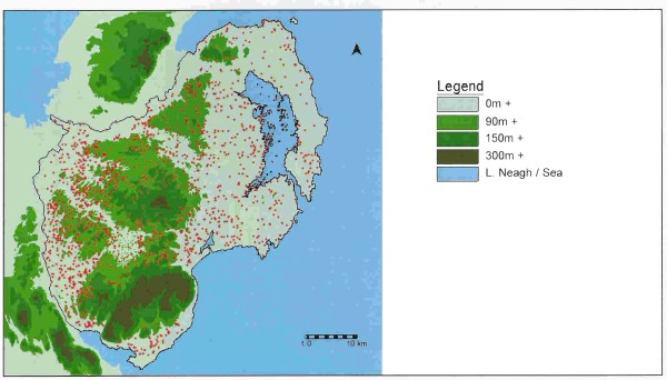
Distribution of Early Christian sites on the contour map

Distribution of Early Christian sites on the contour map

Table 10 shows the number of each site type in each of the soil categories. Again the chi-square test was applied, to highlight any statistically significant results and the results of this can be seen in Table 11.
The number of sites within each soil classification
|
Soil code |
|
|
|
|
|
|
|
|
Principle Soil |
PP (75%) |
ABE (60%) |
ABE (60%) |
ABE (90%) |
Gley (60%) |
ABE (60%) |
|
|
Associated soil |
Peat (25%) |
SBP (40%) |
BP (40%) |
Gley (10%) |
ABE (40%) |
Gley (40%) |
|
|
Rath |
|
|
|
|
|
|
|
|
Probable rath |
|
|
|
|
|
|
|
|
Platform rath |
|
|
|
|
|
|
|
|
Raised rath |
|
|
|
|
|
|
|
|
Rath and souterrain |
|
|
|
|
|
|
|
|
Large rath |
|
|
|
|
|
|
|
|
Conjoined rath |
|
|
|
|
|
|
|
|
Rath pair |
|
|
|
|
|
|
|
|
Bivallate rath |
|
|
|
|
|
|
|
|
Multivallate rath |
|
|
|
|
|
|
|
|
Large enclosure |
|
|
|
|
|
|
|
|
Cashel |
|
|
|
|
|
|
|
|
Crannog |
|
|
|
|
|
|
|
|
Mound |
|
|
|
|
|
|
|
|
Souterrain |
|
|
|
|
|
|
|
|
Ecclesiastical sites |
. |
. |
. |
. |
. |
. |
. |
|
Pre-Viking |
|
|
|
|
|
|
|
|
Pre-Norman |
|
|
|
|
|
|
|
|
Probably pre-Norman |
|
|
|
|
|
|
|
|
Total number of sites |
|
|
|
|
|
|
|
Chi-squared values for each Soil classification
|
Map code |
|
|
|
|
|
19 |
. |
Chi-sq. |
|
Principle soil |
PP (75%) |
ABE (60%) |
ABE (60%) |
ABE (90%) |
Gley (60%) |
ABE (60%) |
Other |
. |
|
Associated soil |
Peat (25%) |
SBP (40%) |
BP (40%) |
Gley (10%) |
ABE (40%) |
Gley (40%) |
. |
. |
|
Rath |
77 |
0.8 |
7 |
1.5 |
43.8 |
41.4 |
77.1 |
248.6 |
|
Probable rath |
3.6 |
0.7 |
0.8 |
1.1 |
0.3 |
5.6 |
3.8 |
16.1 |
|
Platform rath |
2.5 |
0.3 |
0.7 |
0 |
0.1 |
7.4 |
2.7 |
13.7 |
|
Raised rath |
1 |
0 |
6.1 |
0.3 |
0.4 |
0.1 |
1.1 |
9.7 |
|
Rath and souterrain |
0.9 |
1.4 |
1.4 |
0.3 |
0 |
2.2 |
0.9 |
7.2 |
|
Large rath |
0.4 |
1.4 |
1.4 |
0.1 |
17.6 |
1 |
0.4 |
22.1 |
|
Conjoined rath |
0.1 |
5.2 |
0.5 |
0 |
0.4 |
0.3 |
0.1 |
7.5 |
|
Rath pair |
0.7 |
0.7 |
0.7 |
0.2 |
0.4 |
6.5 |
0.7 |
10.3 |
|
Bivallate rath |
1.3 |
0 |
2.6 |
0.9 |
2.2 |
2.5 |
1.4 |
11.4 |
|
Multivallate rath |
0.4 |
0.3 |
0.1 |
0.1 |
1.3 |
3.9 |
0.4 |
7.7 |
|
Large enclosure |
2.3 |
0 |
1.7 |
0.7 |
1.3 |
5.3 |
2.4 |
14.2 |
|
Cashel |
4.3 |
1 |
22.4 |
1.3 |
2 |
4 |
4.5 |
39.8 |
|
Crannog |
1.5 |
0.6 |
0.2 |
0 |
1.1 |
5 |
3.3 |
12.4 |
|
Mound |
0.8 |
0.9 |
0.9 |
0.2 |
0 |
2.5 |
0.8 |
6.1 |
|
Souterrain |
2.2 |
0.7 |
27.6 |
1.2 |
8.4 |
1.3 |
4.1 |
45.2 |
|
Ecclesiastical sites |
. |
. |
. |
. |
. |
. |
. |
. |
|
Pre-Viking |
1.1 |
0.8 |
0.1 |
1.3 |
0 |
2 |
0.6 |
6.9 |
|
Pre-Norman |
0.6 |
9.6 |
3.9 |
1.1 |
0 |
2.9 |
1.2 |
19.4 |
|
Probably pre-Norman |
0.8 |
0.2 |
1.8 |
0.3 |
2.5 |
1.9 |
0 |
8.1 |
Individual values become significant at 3.8
Overall chi-squared vales become significant at 12.59
From this table we can see that many of the site types show a statistically significant preference for the type 15 and 19, acid brown earth / gley soils, of mediocre quality, which is found mostly in the drumlin areas. Only cashels and souterrains indicate an avoidance of these drumlin soil types and a significant preference for the type 6 and 8 brown podzolic / acid brown earth soils, which tend to be found towards the south of the county. Raised raths and conjoined raths are the only other secular site types which demonstrate a statistically significant preference for the brown podzolic / acid brown earth soils, but as we can see from the low chi-squared values in Table 11, this is not a particularly strong preference. The pre-Norman ecclesiastical sites also have a significant preference for the acid brown earth / brown podzolic soil type 6, however, they appear to avoid the type 8 areas. Both Tables 10 and 11 indicate that none of the ecclesiastical sites prefer the acid brown earth / gley soils of the drumlin areas that many of the secular sites do, reflecting the very different distributions of the secular and ecclesiastical settlements. This preference for the better quality soils may support the McCormick’s (1998, 43) suggestion that the church ‘deliberately acquired and maintained land in the (Lecale) area in order to exploit its particular arable qualities’. These results appear to suggest that the church was seeking out the better quality land throughout County Down.
As demonstrated above, the overall preference shown by Early Christian sites in County Down is for settling on acid brown earth / gley soils, with 53% of sites on just 37% of the land (Table 9). These soils, found in the drumlin areas, are of poorer quality, with restricted agricultural use: however, the drumlins tend to have smooth slopes, deep subsoils and natural drainage, which was obviously attractive to the Early Christian settlers (Jope 1966). In his study of County Down, Proudfoot (1957, 456) also found that the distribution of raths could not be explained in terms of better quality soils and studies in other areas in Ireland have revealed similar results, such as County Meath (Brady 1983) County Leitrim (Farrelly 1989, 45) and west mid-Antrim (McErlean 1978, 21). Stout (1997, 93) also notes that the coastal barony of Carbury, within his north-east Connaught zone, includes an area of rolling gley-covered lowlands and has a rath density four times the national average. Although studies in some other areas have found that Early Christian settlements preferred the better quality soils, it is obvious that in numerous areas of Ireland, including County Down, poorer quality, gley soils in drumlin areas were chosen over better quality soil elsewhere. Stout (1997, 107) has summed up the reasons for this as ‘In poorly drained drumlin zones and on wetter upper slopes, gley soils were tolerated; soil quality was traded off against other locational advantages and strategic needs’. In County Down the desire to settle on a drumlin obviously outweighed the considerations of the poorer quality soil this entailed.
Soil categories in each altitude zone
It is obvious from the above results that both soil quality and altitude influenced where Early Christian farmers settled. This raised the question of whether it was possible to determine which attribute exerted the greater influence. To answer this the altitude and soil maps were overlaid to calculate the quantity of each soil type within each altitude zone (Table 12).
Area (km2) of each Soil classification within each altitude zone
|
Soil type |
|
|||||||
|
0 - 30 |
30 - 60 |
60 - 90 |
90 - 150 |
150 - 210 |
210 - 300 |
300 + |
||
|
1 |
PP ( 75%) Peat (25%) |
|
|
|
|
|
|
|
|
6 |
ABE (60%) SBP (40%) |
|
|
|
|
|
|
|
|
8 |
ABE (60%) BP (40%) |
|
|
|
|
|
|
|
|
10 |
ABE (90%) Gley (10%) |
|
|
|
|
|
|
|
|
15 |
Gley (60%) ABE (40%) |
|
|
|
|
|
|
|
|
19 |
ABE (60%) Gley (40%) |
|
|
|
|
|
|
|
|
Other |
Other |
|
|
|
|
|
|
|
Digital elevation model of the County Down Soil Map
The point layer, representing each Early Christian site, was then added to the altitude / Soil map overlay to calculate the number of sites within each category (Table 13) and finally a chi-squared test was applied to highlight any significant correlations and produced the very interesting results which can be seen in Table 14.
Total number of sites within each Soil / altitude category
|
Soil type |
|
|||||||
|
0 - 30 |
30 - 60 |
60 - 90 |
90 - 150 |
150 - 210 |
210 - 300 |
300 + |
||
|
1 |
PP ( 75%) Peat (25%) |
|
|
|
|
|
|
|
|
6 |
ABE (60%) SBP (40%) |
|
|
|
|
|
|
|
|
8 |
ABE (60%) BP (40%) |
|
|
|
|
|
|
|
|
10 |
ABE (90%) Gley (10%) |
|
|
|
|
|
|
|
|
15 |
Gley (60%) ABE (40%) |
|
|
|
|
|
|
|
|
19 |
ABE (60%) Gley (40%) |
|
|
|
|
|
|
|
|
Other |
Other |
|
|
|
|
|
|
|
Chi-squared values for sites within each Soil / altitude category
|
Soil type |
|
|||||||
|
0 - 30 |
30 - 60 |
60 - 90 |
90 - 150 |
150 - 210 |
210 - 300 |
300 + |
||
|
1 |
PP ( 75%) Peat (25%) |
|
|
|
|
|
|
|
|
6 |
ABE (60%) SBP (40%) |
|
0.0 |
|
|
|
|
|
|
8 |
ABE (60%) BP (40%) |
|
|
|
|
|
|
|
|
10 |
ABE (90%) Gley (10%) |
|
|
|
|
|
|
|
|
15 |
Gley (60%) ABE (40%) |
|
|
|
|
|
|
|
|
19 |
ABE (60%) Gley (40%) |
|
|
|
|
|
|
|
|
Other |
Other |
|
|
|
|
|
|
|
(Chi-squared values become significant at 3.8)
From Table 14 we can clearly see that the 60m – 90m zone and particularly the 90m – 150m altitude zone incorporate significantly higher than expected numbers of Early Christian sites. Within the 60m – 90m zone this applies to two of the main soil types and within the 90m – 150m zone there are higher than expected numbers on all four main soil types. This indicates very strongly that altitude was the overriding factor in the location of Early Christian settlement. We can also note from this table, however, that there are significantly high numbers of sites on the very best quality, type 8 (ABE/BP), soil across four altitude zones, ranging from 30m to 210m. This is the only soil type with higher than expected numbers of sites outside the main 60m – 150m settlement zone and indicates that while altitude may have been the dominant factor, exceptions were made, but only for the very best quality, most versatile soil.
Land classification analysis
Figures 14 and 15 below show the distribution of Early Christian sites on the Land Classification map and the summary results of the settlement distribution analysis can be seen in Table 15 below.
|
Quality of Land Classification |
|
|
|
|
|
|
|
High |
|
81.4 |
3.2 |
3 |
0.6 |
0.1 |
|
Medium |
|
389.9 |
15.1 |
16.5 |
0.7 |
2.1 |
|
|
145.8 |
5.7 |
3.5 |
0.4 |
12.4 |
|
|
|
1038.5 |
40.2 |
54.6 |
0.8 |
79 |
|
|
|
341.4 |
13.2 |
13.7 |
0.6 |
0.3 |
|
|
Poor |
|
125.1 |
4.9 |
0.6 |
0.08 |
55.9 |
|
|
17.2 |
0.7 |
0.3 |
0.3 |
2.6 |
|
|
Very poor |
|
106.8 |
4.1 |
0.06 |
0.01 |
61.6 |
|
High/medium |
|
68.8 |
2.7 |
3.7 |
0.8 |
6.4 |
|
|
60.2 |
2.3 |
2.9 |
0.7 |
1.9 |
|
|
Poor/medium |
|
27.9 |
1.1 |
0.4 |
0.2 |
6.8 |
|
Other |
|
177.8 |
6.9 |
0.6 |
0.03 |
88.6 |
(Chi-squared values become significant at 3.8)
From the summary of results we can see that there are two land classes within which Early Christian settlement is particularly dense – A/B1 and B3 at 0.8 per km2. The chi-squared results indicate that these two categories of land, particularly the B3 category, are the only areas with results significantly higher than expected. The vast majority of Early Christian settlement, 54.6%, is found on the B3 land, a rather mediocre quality of land which dominates the drumlin belt area. If we look at the low quality C/B, C and D classes of land, however, the chi-squared results clearly indicate that these areas were being avoided. The density of settlement on this lower-middle class of land confirms what we have already seen in the soil map distribution analysis, i.e. that Early Christian settlements were mostly located on the somewhat poorer quality land, but which was still suitable for the farmers’ needs.
Distribution of Early Christian sites on the Land Classification map
Distribution of Early Christian sites on the Land Classification map
The number of sites within each land classification
|
Land quality |
|
|
|
|
|
|
|
|||||
|
Land classification |
|
|
|
|
|
|
|
|
A / B1 |
A / B2 |
C / B |
Other |
|
Rath |
31 |
195 |
34 |
645 |
129 |
3 |
2 |
0 |
38 |
36 |
4 |
4 |
|
Probable rath |
4 |
11 |
3 |
26 |
4 |
1 |
0 |
0 |
1 |
2 |
0 |
1 |
|
Platform rath |
0 |
6 |
6 |
13 |
7 |
1 |
1 |
0 |
1 |
2 |
0 |
0 |
|
Raised rath |
1 |
2 |
0 |
7 |
2 |
0 |
0 |
0 |
3 |
0 |
0 |
0 |
|
Rath and souterrain |
0 |
1 |
0 |
6 |
5 |
0 |
0 |
0 |
1 |
0 |
0 |
0 |
|
Large rath |
0 |
1 |
1 |
3 |
1 |
0 |
0 |
0 |
0 |
0 |
0 |
0 |
|
Conjoined rath |
0 |
0 |
0 |
2 |
0 |
0 |
0 |
0 |
0 |
0 |
0 |
0 |
|
Rath pair |
0 |
0 |
0 |
8 |
2 |
0 |
0 |
0 |
0 |
0 |
0 |
0 |
|
Bivallate rath |
2 |
3 |
2 |
11 |
1 |
0 |
0 |
0 |
0 |
0 |
0 |
0 |
|
Multivallate rath |
0 |
1 |
0 |
4 |
0 |
0 |
0 |
0 |
0 |
1 |
0 |
0 |
|
Large enclosure |
2 |
4 |
2 |
21 |
2 |
1 |
0 |
0 |
0 |
1 |
0 |
0 |
|
Cashel |
1 |
1 |
0 |
13 |
41 |
3 |
0 |
0 |
3 |
0 |
0 |
0 |
|
Crannog |
1 |
4 |
2 |
30 |
4 |
0 |
0 |
1 |
2 |
1 |
1 |
0 |
|
Mound |
0 |
1 |
1 |
7 |
0 |
0 |
0 |
0 |
2 |
0 |
0 |
0 |
|
Souterrain |
1 |
12 |
1 |
26 |
11 |
0 |
1 |
0 |
4 |
0 |
1 |
0 |
|
Ecclesiastical sites |
|
|
|
|
|
|
|
|
|
|
|
|
|
Pre-Viking |
0 |
4 |
1 |
7 |
0 |
0 |
1 |
0 |
0 |
1 |
0 |
2 |
|
Pre-Norman |
2 |
7 |
1 |
5 |
0 |
0 |
0 |
0 |
1 |
0 |
0 |
1 |
|
Probably pre-Norman |
1 |
1 |
0 |
5 |
2 |
1 |
0 |
0 |
1 |
0 |
0 |
1 |
|
Total no. of sites |
46 |
254 |
54 |
839 |
211 |
10 |
5 |
1 |
57 |
44 |
6 |
9 |
Chi-squared values for each Land classification
|
Land quality |
|
|
|
|
|
|
|
Chi-sq. |
|||||
|
Land Classification |
A |
B1 |
B2 |
B3 |
B4 |
C1 |
C2 |
D |
A/B1 |
A/B2 |
C/B |
Other |
, |
|
Rath |
0.5 |
3.9 |
13.6 |
83.4 |
2.5 |
48.5 |
3.9 |
46.4 |
2.2 |
3.7 |
5.4 |
69.4 |
283.7 |
|
Probable rath |
3.3 |
1.1 |
0 |
1 |
1.3 |
1 |
0.4 |
2.2 |
0.1 |
0.5 |
0.6 |
1.9 |
13.3 |
|
Platform rath |
1.2 |
0 |
7.3 |
0.2 |
0.9 |
0.4 |
2.3 |
1.5 |
0 |
1.5 |
0.4 |
2.6 |
18.3 |
|
Raised rath |
0.6 |
0 |
0.9 |
0.1 |
0 |
0.7 |
0.1 |
0.6 |
16.9 |
0.4 |
0.2 |
1 |
21.6 |
|
Rath and souterrain |
0.4 |
0.5 |
0.73 |
0.1 |
6.3 |
0.6 |
0.1 |
0.5 |
1.2 |
0.3 |
0.1 |
0.9 |
11.8 |
|
Large rath |
0.2 |
0 |
1.3 |
0.1 |
0.1 |
0.3 |
0.1 |
0.3 |
0.2 |
0.1 |
0.1 |
0.4 |
3 |
|
Conjoined rath |
0.1 |
0.3 |
0.1 |
1.8 |
0.3 |
0.1 |
0 |
0.1 |
0.1 |
0 |
0 |
0.1 |
2.9 |
|
Rath pair |
0.3 |
1.5 |
0.6 |
3.9 |
0.4 |
0.5 |
0.1 |
0.4 |
0.3 |
0.2 |
0.1 |
0.7 |
8.9 |
|
Bivallate rath |
3.3 |
0 |
0.8 |
1.5 |
0.9 |
0.9 |
0.1 |
0.8 |
0.5 |
0.4 |
0.2 |
1.3 |
10.8 |
|
Multivallate rath |
0.2 |
0 |
0.3 |
1 |
0.8 |
0.3 |
0 |
0.3 |
0.2 |
5.3 |
0 |
0.4 |
8.9 |
|
Large enclosure |
0.9 |
0.2 |
0 |
4.5 |
1.3 |
0.23 |
0.2 |
1.4 |
0.9 |
0.1 |
0.4 |
2.3 |
12.2 |
|
Cashel |
0.5 |
7.5 |
3.5 |
5.7 |
131 |
0 |
0.4 |
2.6 |
1.1 |
1.4 |
0.7 |
4.3 |
158.7 |
|
Crannog |
0.1 |
1.2 |
0.1 |
7.1 |
0.7 |
2.2 |
0.3 |
0.4 |
0.5 |
0 |
0.5 |
3.2 |
16.5 |
|
Mound |
0.3 |
0.3 |
0.2 |
1.5 |
1.5 |
0.5 |
0.1 |
0.5 |
9.9 |
0.3 |
0.1 |
0.8 |
15.9 |
|
Souterrain |
0.3 |
1.3 |
1.5 |
0.4 |
1.6 |
2.8 |
1 |
2.4 |
4.1 |
1.3 |
0.2 |
3.9 |
20.9 |
|
Ecclesiastical sites |
. |
||||||||||||
|
Pre-Viking |
0.5 |
1 |
0 |
0 |
2.1 |
0.8 |
7.6 |
0.7 |
0.4 |
1 |
0.2 |
0.7 |
15.1 |
|
Pre-Norman |
4 |
7.6 |
0 |
0.5 |
2.3 |
0.8 |
0.1 |
0.7 |
0.7 |
0.4 |
0.2 |
0 |
17.3 |
|
Probably pre-Norman |
1 |
0.4 |
0.7 |
0 |
0.1 |
0.3 |
0.1 |
0.5 |
1.5 |
0.3 |
0.1 |
0 |
4.9 |
Individual values become significant at 3.8 Overall chi-squared vales become significant at 19.68
Table 16 shows the distribution of each site type on the various categories of land and the results of applying a chi-squared test to this are in Table 17. From this we can see that raised raths, multivallate raths, mounds and souterrains demonstrate statistically significant preferences for the high quality A/B1 and A/B2 categories of land. This may support the suggestion by Mytum (1992, 126) and Avery (1991, 125) that raised raths are high status sites and multivallate raths are also considered to be high status. These results also suggest that at least some of the mounds may actually be raised raths. The B3 category also produces a number of statistically significant results, indicating concentrations of rath pairs, large enclosures, crannog and particularly raths. This B3 category of land dominates the drumlin belt and again this explains the concentration of raths in this category. Particularly significant, however, are the chi-squared results for the C/B, C1, C2 and D categories which confirm the summary results (Table 15) and clearly demonstrate that Early Christian rath builders were carefully avoiding these poor quality areas, as we would expect from an agricultural based society. Only cashels have results which are significantly lower than expected in both the B1 and B3 categories and higher in the poorer quality B4 classification, reflecting the upland distribution of these settlements. The pre-Viking ecclesiastical sites also have a surprisingly high occurrence in the poor quality, C category of land. By contrast the pre-Norman ecclesiastical sites are the only site type to have a higher than expected number of sites in the highest quality, A category and, as they achieve the same in the B1 category, we must assume that they were deliberately located on the best quality land, capable of growing crops. This result is not reflected in either the pre-Viking or probably pre-Norman ecclesiastical site types.
Overall, Table 17 demonstrates that there is a low site density on the land of B4 or poorer quality while, above this, we can see quite a number of statistically significant clusters of sites. As with the soil analysis, raths, the dominant settlement form of the period, are concentrated on the B3, lower-middle quality land.
Land Classification categories in each altitude zone
As with the Soil map, the Land Classification map was overlaid with the altitude map to calculate the quantity of each classification within each altitude zone (Table 18).
Figure 16
Digital elevation model of the County Down Land Classification map